How to Do Conjoint Analysis in python

#statistics

This post shows how to do conjoint analysis using python. Conjoint analysis is a method to find the most prefered settings of a product [11].

Usual fields of usage [3]:

Marketing
Product management
Operation Research

For example:

testing customer acceptance of new product design.
assessing appeal of advertisements and service design.

import pandas as pd
import numpy as np

Here we used Immigrant conjoint data described by [6]. It consists of 2 possible conjoint methods: choice-based conjoint (with selected column as target variable) and rating-based conjoint (with rating as target variable).

Preparing The Data

# taken from imigrant conjoint data
df = pd.read_csv('https://dataverse.harvard.edu/api/access/datafile/2445996?format=tab&gbrecs=true', delimiter='\t')

df.head()

	resID	atmilitary	atreligion	ated	atprof	atinc	atrace	atage	atmale	selected	rating
0	383	1	6	3	6	6	1	6	2	0	0.333333
1	383	2	1	1	4	3	6	4	1	1	0.500000
2	383	1	3	5	5	1	2	5	2	1	0.666667
3	383	2	4	5	3	2	1	6	1	0	0.666667
4	383	2	1	2	3	6	2	2	2	0	0.333333

# checking for empty data
df.isnull().sum()

resID          0
atmilitary     0
atreligion     0
ated           0
atprof         0
atinc          0
atrace         0
atage          0
atmale         0
selected       0
rating        10
dtype: int64

# remove empty data
clean_df = df[~df.rating.isnull()]

Doing The Conjoint Analysis

y = clean_df['selected']
x = clean_df[[x for x in df.columns if x != 'selected' and x != 'resID' and x != 'rating']]

xdum = pd.get_dummies(x, columns=[c for c in x.columns if c != 'selected'])
xdum.head()

	atmilitary_1	atmilitary_2	atreligion_1	atreligion_3	atreligion_4	atreligion_6	ated_1	ated_2	...	atrace_6	atage_2	atage_4	atage_5	atage_6	atmale_1	atmale_2
0	1	0	0	0	0	1	0	0	...	0	0	0	0	1	0	1
1	0	1	1	0	0	0	1	0	...	1	0	1	0	0	1	0
2	1	0	0	1	0	0	0	0	...	0	0	0	1	0	0	1
3	0	1	0	0	1	0	0	0	...	0	0	0	0	1	1	0
4	0	1	1	0	0	0	0	1	...	0	1	0	0	0	0	1

5 rows × 40 columns

[11] has complete definition of important attributes in Conjoint Analysis

Utility of an alternative $U(x)$ is

\[U(x) = \sum_{i=1}^{m}\sum_{j=1}^{k_{i}}u_{ij}x_{ij}\]

where:

$u_{ij}$: part-worth contribution (utility of jth level of ith attribute)

$k_{i}$: number of levels for attribute i

$m$: number of attributes

Importance of an attribute $R_{i}$ is defined as $R_{i} = max(u_{ij}) - min(u_{ik})$ $R_{i}$ is the $i$-th attribute

Relative Importance of an attribute $Rimp_{i}$ is defined as $Rimp_{i} = \frac{R_{i}}{\sum_{i=1}^{m}{R_{i}}}$

Essentially conjoint analysis (traditional conjoint analysis) is doing linear regression where the target variable could be binary (choice-based conjoint analysis), or 1-7 likert scale (rating conjoint analysis), or ranking(rank-based conjoint analysis).

import statsmodels.api as sm
import seaborn as sns
import matplotlib.pyplot as plt
plt.style.use('bmh')

res = sm.OLS(y, xdum, family=sm.families.Binomial()).fit()
res.summary()

OLS Regression Results
Dep. Variable:	selected	R-squared:	0.091
Model:	OLS	Adj. R-squared:	0.083
Method:	Least Squares	F-statistic:	10.72
Date:	Sun, 09 Dec 2018	Prob (F-statistic):	7.39e-51
Time:	15:49:37	Log-Likelihood:	-2343.3
No. Observations:	3456	AIC:	4753.
Df Residuals:	3423	BIC:	4956.
Df Model:	32
Covariance Type:	nonrobust

	coef	std err	t	P>\|t\|	[0.025	0.975]
atmilitary_1	0.0808	0.008	9.585	0.000	0.064	0.097
atmilitary_2	0.1671	0.008	19.810	0.000	0.151	0.184
atreligion_1	0.0931	0.018	5.132	0.000	0.058	0.129
atreligion_2	0.0578	0.018	3.144	0.002	0.022	0.094
atreligion_3	0.0803	0.018	4.411	0.000	0.045	0.116
atreligion_4	0.0797	0.018	4.326	0.000	0.044	0.116
atreligion_5	-0.0218	0.018	-1.185	0.236	-0.058	0.014
atreligion_6	-0.0411	0.018	-2.256	0.024	-0.077	-0.005
ated_1	-0.1124	0.018	-6.115	0.000	-0.148	-0.076
ated_2	0.0278	0.019	1.464	0.143	-0.009	0.065
ated_3	0.0366	0.019	1.942	0.052	-0.000	0.074
ated_4	0.0737	0.018	4.076	0.000	0.038	0.109
ated_5	0.0649	0.018	3.570	0.000	0.029	0.101
ated_6	0.1572	0.018	8.949	0.000	0.123	0.192
atprof_1	0.1084	0.018	5.930	0.000	0.073	0.144
atprof_2	0.0852	0.019	4.597	0.000	0.049	0.122
atprof_3	0.0910	0.018	5.060	0.000	0.056	0.126
atprof_4	0.0674	0.018	3.716	0.000	0.032	0.103
atprof_5	0.0145	0.019	0.779	0.436	-0.022	0.051
atprof_6	-0.1186	0.018	-6.465	0.000	-0.155	-0.083
atinc_1	0.0081	0.018	0.448	0.654	-0.027	0.043
atinc_2	0.0316	0.019	1.662	0.097	-0.006	0.069
atinc_3	0.0716	0.018	4.020	0.000	0.037	0.106
atinc_4	0.0397	0.018	2.154	0.031	0.004	0.076
atinc_5	0.0808	0.018	4.451	0.000	0.045	0.116
atinc_6	0.0161	0.018	0.872	0.383	-0.020	0.052
atrace_1	0.0274	0.018	1.494	0.135	-0.009	0.063
atrace_2	0.0527	0.018	2.881	0.004	0.017	0.089
atrace_3	0.0633	0.018	3.556	0.000	0.028	0.098
atrace_4	0.0037	0.019	0.198	0.843	-0.033	0.040
atrace_5	0.0324	0.018	1.787	0.074	-0.003	0.068
atrace_6	0.0683	0.019	3.687	0.000	0.032	0.105
atage_1	0.0680	0.018	3.770	0.000	0.033	0.103
atage_2	0.0934	0.019	4.957	0.000	0.056	0.130
atage_3	0.0900	0.018	4.967	0.000	0.054	0.125
atage_4	0.0711	0.019	3.837	0.000	0.035	0.107
atage_5	0.0038	0.018	0.208	0.835	-0.032	0.039
atage_6	-0.0783	0.018	-4.276	0.000	-0.114	-0.042
atmale_1	0.1228	0.008	14.616	0.000	0.106	0.139
atmale_2	0.1250	0.008	14.787	0.000	0.108	0.142

Omnibus:	0.070	Durbin-Watson:	2.872
Prob(Omnibus):	0.966	Jarque-Bera (JB):	391.306
Skew:	-0.011	Prob(JB):	1.07e-85
Kurtosis:	1.352	Cond. No.	1.27e+16

Warnings:
[1] Standard Errors assume that the covariance matrix of the errors is correctly specified.
[2] The smallest eigenvalue is 4.28e-29. This might indicate that there are
strong multicollinearity problems or that the design matrix is singular.

df_res = pd.DataFrame({
    'param_name': res.params.keys()
    , 'param_w': res.params.values
    , 'pval': res.pvalues
})
# adding field for absolute of parameters
df_res['abs_param_w'] = np.abs(df_res['param_w'])
# marking field is significant under 95% confidence interval
df_res['is_sig_95'] = (df_res['pval'] < 0.05)
# constructing color naming for each param
df_res['c'] = ['blue' if x else 'red' for x in df_res['is_sig_95']]

# make it sorted by abs of parameter value
df_res = df_res.sort_values(by='abs_param_w', ascending=True)

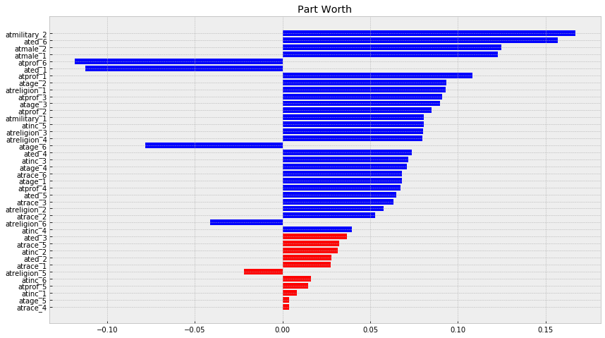
f, ax = plt.subplots(figsize=(14, 8))
plt.title('Part Worth')
pwu = df_res['param_w']
xbar = np.arange(len(pwu))
plt.barh(xbar, pwu, color=df_res['c'])
plt.yticks(xbar, labels=df_res['param_name'])
plt.show()

png

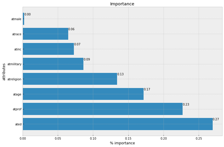
Now we will compute importance of every attributes, with definition from before, where:

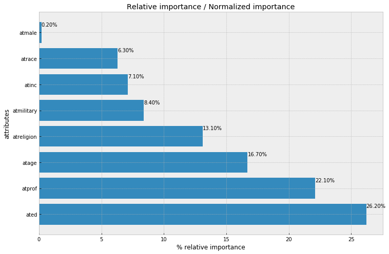
\[R_{i} = max(u_{ij}) - min(u_{ik})\] \[Rimp_{i} = \frac{R_{i}}{\sum_{i=1}^{m}{R_{i}}}\]

sum of importance on attributes will approximately equal to the target variable scale: if it is choice-based then it will equal to 1, if it is likert scale 1-7 it will equal to 7. In this case, importance of an attribute will equal with relative importance of an attribute because it is choice-based conjoint analysis (the target variable is binary).

# need to assemble per attribute for every level of that attribute in dicionary
range_per_feature = dict()
for key, coeff in res.params.items():
    sk =  key.split('_')
    feature = sk[0]
    if len(sk) == 1:
        feature = key
    if feature not in range_per_feature:
        range_per_feature[feature] = list()
        
    range_per_feature[feature].append(coeff)

# importance per feature is range of coef in a feature
# while range is simply max(x) - min(x)
importance_per_feature = {
    k: max(v) - min(v) for k, v in range_per_feature.items()
}

# compute relative importance per feature
# or normalized feature importance by dividing 
# sum of importance for all features
total_feature_importance = sum(importance_per_feature.values())
relative_importance_per_feature = {
    k: 100 * round(v/total_feature_importance, 3) for k, v in importance_per_feature.items()
}

alt_data = pd.DataFrame(
    list(importance_per_feature.items()), 
    columns=['attr', 'importance']
).sort_values(by='importance', ascending=False)


f, ax = plt.subplots(figsize=(12, 8))
xbar = np.arange(len(alt_data['attr']))
plt.title('Importance')
plt.barh(xbar, alt_data['importance'])
for i, v in enumerate(alt_data['importance']):
    ax.text(v , i + .25, '{:.2f}'.format(v))
plt.ylabel('attributes')
plt.xlabel('% importance')
plt.yticks(xbar, alt_data['attr'])
plt.show()

png

alt_data = pd.DataFrame(
    list(relative_importance_per_feature.items()), 
    columns=['attr', 'relative_importance (pct)']
).sort_values(by='relative_importance (pct)', ascending=False)


f, ax = plt.subplots(figsize=(12, 8))
xbar = np.arange(len(alt_data['attr']))
plt.title('Relative importance / Normalized importance')
plt.barh(xbar, alt_data['relative_importance (pct)'])
for i, v in enumerate(alt_data['relative_importance (pct)']):
    ax.text(v , i + .25, '{:.2f}%'.format(v))
plt.ylabel('attributes')
plt.xlabel('% relative importance')
plt.yticks(xbar, alt_data['attr'])
plt.show()